
Evaluating a wearable or staging algorithm against a reference#
How good is a wearable, or a sleep staging algorithm, at scoring sleep? To find out, we need to compare it against polysomnography (PSG), the gold standard. This tutorial shows how to do this with YASA, following the standardized framework of Menghini et al. (2021). We use the same data and the same steps as the authors’ R analytical pipeline, in just a few lines of Python.
The evaluation has two parts, each handled by a dedicated class in the YASA API:
Epoch-by-epoch agreement (
EpochByEpochAgreement). Does the device assign the right stage to each 30-second epoch? This part tells you where and why the device goes wrong.Sleep statistics agreement (
SleepStatsAgreement). Does the device get the nightly summaries right, such as total sleep time or minutes of REM sleep? This part tells you how much these errors matter.
Throughout the tutorial, the “device” is the sleep tracker or sleep staging algorithm that we want to evaluate, and the “reference” is the method we compare it against, usually expert scoring of PSG data.
The data#
We’ll use the sample dataset of the R pipeline. It contains one night from each of 14 healthy adults, recorded in the SRI human sleep laboratory, representing 10,766 epochs of 30 seconds in total. Each night was scored at the same time by PSG, following the AASM criteria, and by a consumer wrist-worn device. Stages are coded as integers: 0 = Wake, 1 = Light (N1 + N2), 2 = Deep (N3) and 3 = REM.
>>> import pandas as pd
>>> import yasa
>>> url = "https://github.com/raphaelvallat/yasa/raw/master/tests/data/sample_data_sri.csv.xz"
>>> df = pd.read_csv(url)
>>> df.head(3)
  subject  epoch  reference  device
0   sbj01      1          0       0
1   sbj01      2          0       0
2   sbj01      3          0       0
The data is in the “long” format: there is one row per epoch, one column for the subject, one for the epoch, and one for each scoring method.
Let’s turn each night into a pair of 4-stage Hypnogram objects, one per scorer. YASA
uses the scorer name to tell the reference from the device in all its outputs:
>>> mapping = {0: "WAKE", 1: "LIGHT", 2: "DEEP", 3: "REM"}
>>> ref_hyps, obs_hyps = {}, {}
>>> for sub, d in df.groupby("subject"):
...     ref_hyps[sub] = yasa.Hypnogram.from_integers(
...         d["reference"], mapping=mapping, n_stages=4, scorer="PSG"
...     )
...     obs_hyps[sub] = yasa.Hypnogram.from_integers(
...         d["device"], mapping=mapping, n_stages=4, scorer="Device"
...     )
>>> ref_hyps["sbj01"]
<Hypnogram | 882 epochs x 30s (441.00 minutes), 4 unique stages, scored by PSG>
Note
To compare just two hypnograms, you don’t need the dictionaries. Simply use
ref_hyp.evaluate(obs_hyp) (see Hypnogram.evaluate).
Our dataset has one night per subject. If you have several nights per subject, give each night
its own key (e.g. "sbj01_night1"). Keep in mind that the group-level metrics and confidence
intervals will then treat each night as independent.
Data requirements#
Before running the analyses, make sure that your data meets the following conditions:
Simultaneous recordings. The device and the reference measured the same night, at the same time.
Same epoch length. Both recordings use the same epoch length, e.g. 30 seconds. Ideally, this is the resolution that the device’s algorithm was designed for.
Same recording bounds. Both recordings cover the same time in bed, from lights-off to lights-on.
Synchronization. The two recordings are aligned epoch by epoch. This is important, because even a small offset can substantially degrade the epoch-by-epoch metrics.
Same coding system. Both recordings use the same stages. Most consumer devices report “light” sleep for PSG N1 + N2 and “deep” sleep for PSG N3.
No missing data. Every epoch has a value for both the device and the reference.
Proper use. The device was worn as recommended by the manufacturer, e.g. its fit and placement.
YASA checks some of these for you. Each pair of hypnograms must have the same number of epochs, and all hypnograms must share the same epoch length and stage labels.
Part 1: Epoch-by-epoch agreement#
Epoch-by-epoch (EBE) analysis assesses how well a device classifies sleep stages. Because it compares the two hypnograms epoch by epoch, it requires a device that lets you export its epoch-level data. If yours only provides nightly summaries, skip to Part 2.
In YASA, we initiate the EBE analysis with:
>>> ebe = yasa.EpochByEpochAgreement(ref_hyps, obs_hyps)
>>> ebe
<EpochByEpochAgreement | Observed hypnograms scored by Device evaluated against reference
hypnograms scored by PSG, 14 sleep sessions>
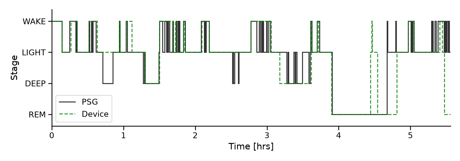
Before computing any metric, it is a good idea to look at the data. We can plot the hypnograms of the device and reference with:
>>> ebe.plot_hypnograms(sleep_id="sbj03")
Error matrix#
The error matrix, also known as the confusion matrix, shows where the device goes wrong.
Rows are PSG stages and columns are device stages. Each cell counts the epochs that fall into
that combination. For example, the cell at the DEEP row and LIGHT column counts the
epochs scored as deep sleep by PSG but as light sleep by the device. Summing the epochs of all
nights gives the absolute error matrix:
>>> ebe.get_confusion_matrix(agg_func="sum")
Device  WAKE  LIGHT  DEEP  REM
PSG
WAKE     871    483    29   71
LIGHT    303   4381   398  521
DEEP      34   1142   925   16
REM       57    564    49  922
This matrix is easy to compute but can be hard to interpret. Raw counts are dominated by the most common stage (light sleep) and by the longest nights. In addition, pooling all nights gives a single number per cell and hides how much the device varies from one person to the next.
This is why Menghini et al. recommend the proportional error matrix. First, a matrix is computed for each night, and each row is expressed as a percentage of the PSG epochs of that stage. The individual matrices are then averaged across nights, and each cell is reported with its SD and 95% confidence interval. Here, the confidence intervals are obtained by bootstrapping the nights. This per-night matrix is required in all performance evaluation papers submitted to the journal Sleep Health (de Zambotti et al., 2022).
>>> boot = {"method": "percentile", "rng": 42}
>>> cm = ebe.get_confusion_matrix_proportional(bootstrap_kwargs=boot)
>>> cm.round(1).head(4)
             mean   std  ci_lower  ci_upper  n_sessions
PSG  Device
WAKE WAKE    61.9  16.2      53.4      69.5          14
     LIGHT   30.6  17.6      22.6      39.9          14
     DEEP     1.9   2.5       0.8       3.3          14
     REM      5.5  10.4       1.5      11.4          14
Tip
Setting a seed ("rng": 42) makes the bootstrap confidence intervals reproducible. The
default bootstrap method, BCa, works best with large samples and can be unstable with few
nights. With only 14 nights, we use the simple "percentile" method throughout this tutorial.
Use formatted=True to get a publication-ready table with mean (SD) [CI] in each cell. For
a quick overview, a heatmap of the means works best:
>>> import seaborn as sns
>>> stages = ["WAKE", "LIGHT", "DEEP", "REM"]
>>> mat = cm["mean"].unstack().loc[stages, stages]
>>> sns.heatmap(mat, annot=True, fmt=".1f", cmap="Blues", vmin=0, vmax=100, square=True)
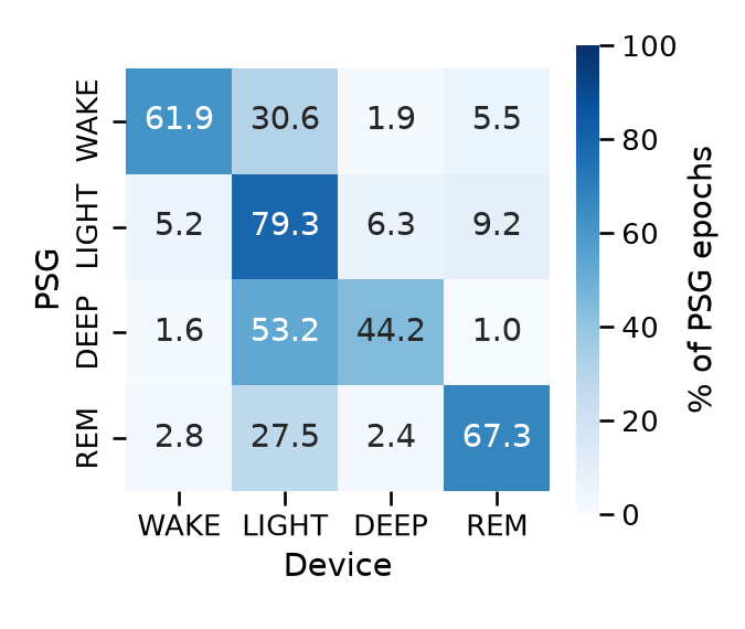
The diagonal is the percentage of epochs that the device got right, which is the sensitivity of each stage.
The device recognizes light sleep well, with about 80% of PSG N1 + N2 epochs correctly classified. Deep sleep is a different story: more than half of the PSG N3 epochs end up as light sleep. Wake (31%) and REM sleep (27%) are also frequently mistaken for light sleep. This is where most of the device’s errors go, and as we’ll see in Part 2, it overestimates light sleep as a result.
Note that the SD and the confidence interval answer two different questions:
The SD tells you how much nights differ from each other. Deep and REM sensitivities vary a lot between participants, with SDs of 24% and 33%, respectively.
The confidence interval tells you how precisely we know the group mean. The percentage of light sleep scored as wake is estimated precisely (5.2%, CI: 3.7–6.9%). Deep sensitivity (44%, CI: 33–57%) and REM sensitivity (67%, CI: 50–84%) are much less certain and should be interpreted with caution.
Overall agreement#
get_agreement returns one row of agreement scores per night.
summary then aggregates them across nights. Add
ci_method="boot" to get a bootstrap confidence interval of the mean:
>>> ebe.get_agreement().round(2).head(3)
          accuracy  balanced_acc  kappa   mcc  precision     f1
sleep_id
sbj01        61.34         51.86   0.31  0.32      59.21  57.09
sbj02        59.06         50.52   0.31  0.37      62.22  52.08
sbj03        76.16         76.53   0.62  0.63      77.25  76.37

>>> summ = ebe.summary(ci_method="boot", bootstrap_kwargs=boot)
>>> summ[["mean", "std", "ci_lower", "ci_upper"]].round(2)
               mean   std  ci_lower  ci_upper
metric
accuracy      66.18  6.60     62.83     69.51
balanced_acc  63.18  8.73     58.87     67.53
kappa          0.45  0.12      0.39      0.51
mcc            0.47  0.12      0.42      0.53
precision     69.53  8.28     65.26     73.54
f1            64.53  8.19     60.37     68.64
On average, the device agrees with PSG on two out of three epochs (66% accuracy). The other scores look at the agreement from different angles:
Cohen’s kappa (0.45) measures the agreement beyond what we would expect by chance. Its value depends on the number of stages and on how common each stage is.
Balanced accuracy is the average sensitivity across stages (macro-average, i.e. each stage counts equally regardless of its duration).
The other scores are described in get_agreement.
Warning
Avoid reporting accuracy alone. Sleep stages are typically imbalanced, and a device can reach a high accuracy while missing most epochs of a less frequent stage. Report it together with the sensitivity and specificity of each stage (see below).
Agreement by stage#
Overall scores can hide large errors in specific stages. To see them,
get_agreement_bystage computes metrics for each stage and each
night. As before, summary(by_stage=True) averages them across nights.
In sleep/wake classification, sensitivity is defined as the ability to detect sleep and specificity as the ability to detect wake. With more stages, sensitivity is the ability of the device to detect a given stage (e.g. REM), while specificity is its ability to reject all the other stages. YASA uses the scikit-learn names for these classification metrics:
YASA |
Menghini et al. |
Definition, for a given stage |
|---|---|---|
|
Sensitivity |
% of the PSG epochs of this stage that the device correctly classifies as this stage |
|
Specificity |
% of the PSG epochs of other stages that the device correctly does not classify as this stage |
|
Positive predictive value (PPV) |
% of the epochs classified as this stage by the device that are this stage in the PSG |
|
Negative predictive value (NPV) |
% of the epochs not classified as this stage by the device that are not this stage in the PSG |
>>> summ = ebe.summary(by_stage=True)
>>> metrics = ["recall", "specificity", "precision", "npv"]
>>> summ["mean"].unstack("stage").loc[metrics, stages].round(1)
stage        WAKE  LIGHT  DEEP   REM
metric
recall       61.9   79.3  44.2  67.3
specificity  95.9   58.4  94.9  93.6
precision    68.1   67.7  66.1  62.2
npv          93.7   73.0  87.2  93.4
The recall row is simply the diagonal of the proportional error matrix. Specificity is above 90% for all stages except light sleep (58%). This is the flip side of what we saw earlier: because the device over-scores light sleep, it often says “light” when the reference PSG says otherwise.
Note
If a night has no epoch of a given stage in the PSG (e.g. no deep sleep), the recall of that
stage is undefined for that night. YASA leaves it as NaN to avoid pulling the group mean
down. Use get_agreement_bystage(zero_division=0) to count it as 0% instead.
Sleep vs wake#
Many devices, including standard actigraphy, only distinguish sleep from wake. To evaluate them,
merge Light, Deep and REM into a single SLEEP stage with
Hypnogram.consolidate_stages:
>>> ref_sw = {k: h.consolidate_stages(2) for k, h in ref_hyps.items()}
>>> obs_sw = {k: h.consolidate_stages(2) for k, h in obs_hyps.items()}
>>> ebe_sw = yasa.EpochByEpochAgreement(ref_sw, obs_sw)
>>> ebe_sw.summary().loc[["accuracy", "kappa"], ["mean", "std"]].round(2)
           mean   std
metric
accuracy  90.82  3.90
kappa      0.58  0.14

>>> sleep = ebe_sw.summary(by_stage=True).loc["SLEEP"]
>>> sleep.loc[["recall", "specificity"], ["mean", "std"]].round(1)
             mean   std
metric
recall       95.9   2.3
specificity  61.9  16.2
With only two stages, the metrics of one stage mirror those of the other. The specificity of sleep is the sensitivity of wake, and vice versa. The device detects 96% of the sleep epochs, but only 62% of the wake epochs.
Part 2: Sleep statistics agreement#
In the second part, we move from epochs to nights. How far are the device’s nightly sleep statistics from those of the reference? This discrepancy analysis doesn’t need epoch-by-epoch data. It is also directly relevant if you plan to use the device in a study, for example to measure total sleep time.
get_sleep_stats computes the sleep statistics of every night,
for both scorers:
>>> sstats = ebe.get_sleep_stats()
>>> stats = ["TST", "SE", "SOL", "WASO", "LIGHT", "DEEP", "REM"]
>>> sstats.loc["Device", stats].head(3).round(1)
            TST    SE   SOL  WASO  LIGHT  DEEP   REM
sleep_id
sbj01     378.0  85.7  22.0  41.0  315.0  39.5  23.5
sbj02     354.5  89.9   7.5  32.5  312.0  26.5  16.0
sbj03     262.5  78.7   8.5  62.5  170.5  38.5  53.5
All durations are in minutes. SleepStatsAgreement takes this table as is, and runs a
Bland-Altman analysis on every statistic. Statistics that are identical between the two scorers,
such as the time in bed, are dropped.
>>> ssa = yasa.SleepStatsAgreement(sstats, bootstrap_kwargs=boot)
>>> ssa
<SleepStatsAgreement | Observed scorer ('Device') evaluated against reference scorer ('PSG'),
14 sleep sessions>
Bias and limits of agreement#
For each night, we compute the difference device − reference. A positive difference means that the device overestimates the statistic, and a negative difference means that it underestimates it. Following Bland and Altman, we then summarize these differences into the two components of the device’s measurement error:
The bias is the systematic error, i.e. the average difference between the device and the reference. If its confidence interval excludes zero, the device consistently over- or underestimates the statistic.
The 95% limits of agreement (LoA) describe the random error. For a new night, we expect the difference to fall within these limits 95% of the time.
Both are expressed in the unit of the statistic, e.g. minutes. This makes them easier to interpret than a correlation coefficient. A correlation measures the association between two methods, not their agreement. Two measures of total sleep time that always differ by 50 minutes are perfectly correlated, even though they never agree.
report computes both for every statistic, in the table recommended
by Menghini et al. For each statistic, it shows the mean (SD) of each scorer, the bias and LoA
with their 95% confidence intervals, and the outcome of the assumption tests:
>>> report = ssa.report(sleep_stats=stats)
>>> report[["PSG mean (SD)", "Device mean (SD)", "Bias [95% CI]"]]
              PSG mean (SD) Device mean (SD)                                         Bias [95% CI]
sleep_stat
TST (min)    332.57 (67.25)   339.32 (60.61)                                   6.75 [-6.19, 19.69]
SE (%)         86.08 (6.90)     88.07 (4.53)   58.10 + -0.65x [b0: 15.69, 85.54; b1: -0.97, -0.18]
SOL (min)     13.75 (11.60)    11.36 (14.81)                                  -2.39 [-11.43, 5.14]
WASO (min)    36.18 (21.19)    33.29 (12.57)    25.55 + -0.79x [b0: 8.16, 38.75; b1: -1.24, -0.10]
LIGHT (min)  200.11 (48.52)   234.64 (56.85)                                   34.54 [4.01, 65.06]
DEEP (min)    75.61 (23.71)    50.04 (22.58)  23.70 + -0.65x [b0: -20.32, 67.72; b1: -1.21, -0.09]
REM (min)     56.86 (23.11)    54.64 (27.39)  56.14 + -1.03x [b0: 10.63, 101.66; b1: -1.77, -0.28]

>>> report[["LoA [95% CI]", "Assumptions"]]
                                                            LoA [95% CI]                                 Assumptions
sleep_stat
TST (min)                 -37.16 to 50.66 [-59.57, -14.76; 28.26, 73.07]  ✓ normal  ✓ constant bias  ✓ homoscedastic
SE (%)       ±2.46 (24.90 + -0.26x) [c0: 13.44, 36.70; c1: -0.39, -0.13]  ✗ normal  ✗ constant bias  ✗ homoscedastic
SOL (min)                 -34.69 to 29.90 [-48.39, -11.58; 10.54, 46.16]  ✗ normal  ✓ constant bias  ✓ homoscedastic
WASO (min)                                   bias ± 22.98 [11.14, 30.45]  ✗ normal  ✗ constant bias  ✓ homoscedastic
LIGHT (min)            -69.08 to 138.15 [-121.94, -16.21; 85.28, 191.01]  ✓ normal  ✓ constant bias  ✓ homoscedastic
DEEP (min)                                   bias ± 41.18 [24.23, 58.14]  ✓ normal  ✗ constant bias  ✓ homoscedastic
REM (min)                                    bias ± 53.68 [31.57, 75.78]  ✓ normal  ✗ constant bias  ✓ homoscedastic
Let’s start with the rows where the bias and the LoA are single numbers:
Total sleep time is well estimated on average. The bias is only +7 minutes, and its confidence interval includes zero. However, the LoA are wide. On a given night, the device can be anywhere from 37 minutes below to 51 minutes above PSG.
Light sleep is overestimated. The bias is positive, and its confidence interval is entirely above zero. We could correct this systematic error by subtracting 34.54 minutes (the “calibration index”) from the device’s light sleep. But calibration does not reduce the random error, and the LoA still span more than 3 hours.
Sleep onset latency is also unbiased on average (−2 minutes), but its LoA span more than an hour, for a statistic that averages about 14 minutes in the PSG.
The other rows show equations instead of single numbers, and some assumptions are marked as not met (✗). To understand why, let’s look at the data.
Bland-Altman plots#
The Bland-Altman plot is a widely used way to visualize the agreement between two methods.
plot_blandaltman plots the differences against the PSG values.
The solid line is the bias and the dashed lines are the LoA, each with its confidence band:
>>> ssa.plot_blandaltman(sleep_stats=["TST", "WASO", "DEEP", "REM"], col_wrap=2)
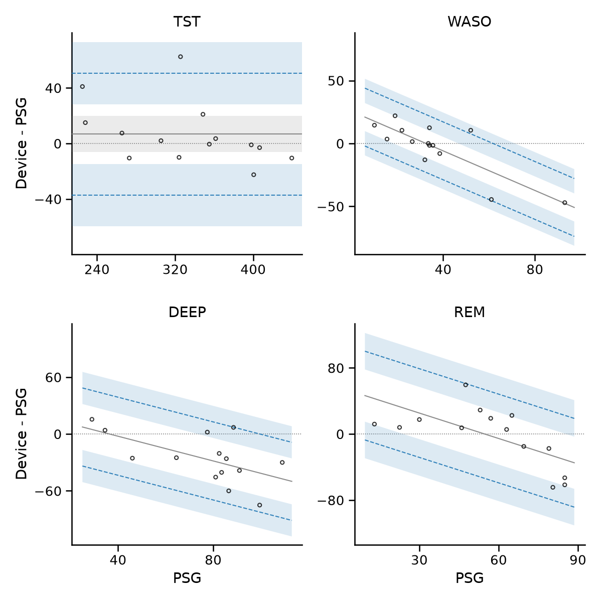
To interpret these results, we first need to understand the three assumptions behind the Bland-Altman method (Bland and Altman, 1999):
The bias does not vary with the reference values, e.g. the bias remains constant as total sleep time (TST) increases.
The random error is the same across the range of reference values (homoscedasticity).
The differences are normally distributed.
Like the R pipeline, YASA tests each assumption for each statistic, and adapts the method when an assumption is not met.
Assumption 1: Constant bias. YASA regresses the differences on the PSG values:
If the slope \(b_1\) is significant, the bias is proportional. It is then reported as this regression line, rather than as a mean difference. In the report above, the bias for deep sleep is \(23.70 - 0.65 \times \text{PSG}\), meaning that on a night with 75 minutes of deep sleep (the group average), the device underestimates deep sleep by about 25 minutes, whereas on a night with only 36 minutes, it is right on average. The LoA then run parallel to the bias line, at \(\pm 1.96\) SD of the regression residuals.
Assumption 2: Homoscedasticity. YASA regresses the absolute residuals of the bias model (\(AR\)) on the PSG values:
If the slope \(c_1\) is significant, the differences are heteroscedastic. Their spread increases or decreases with the size of the measurement, and so do the LoA:
Here, \(c_0 + c_1 \, \text{PSG}\) is the average distance between the nights and the bias line at a given PSG value, and the factor 2.46 turns this average distance into limits of agreement (see the panel below for details).
Let’s take sleep efficiency (SE) as an example. In the report above, SE has a proportional bias, 58.10 + -0.65x, and heteroscedastic LoA, ±2.46 (24.90 + -0.26x), where x is the PSG value. To get the LoA on a night with a PSG sleep efficiency of 80%:
Bias: 58.10 − 0.65 × 80 = 6.10. On average, the device reports a sleep efficiency of about 86% instead of 80%.
Average distance to the bias line: 24.90 − 0.26 × 80 = 4.10.
Half-width of the LoA: 2.46 × 4.10 = 10.09.
LoA: 6.10 ± 10.09, i.e. from −3.99 to +16.19. Adding these limits to the PSG value, we expect the device to report a sleep efficiency between 76% and 96% on 95% of the nights with a PSG sleep efficiency of 80%.
On a night with a PSG sleep efficiency of 90%, the same steps give a bias of −0.40 and LoA from −4.09 to +3.29, i.e. a device value between 86% and 93%. This range is almost three times narrower than at 80%. In other words, the device is less reliable on nights of poor sleep.
Where does the factor 2.46 come from?
The usual LoA are placed at 1.96 standard deviations (SD) on either side of the bias. When the differences are heteroscedastic, there is no longer a single SD, because the spread changes with the PSG value. YASA estimates this spread from the absolute residuals, i.e. how far each night falls from the bias line, ignoring whether it is above or below. The regression \(c_0 + c_1 \, \text{PSG}\) then gives the average distance to the bias line for any PSG value.
The average distance and the SD both measure spread, but they are not equal. For normally distributed data, the average distance to the center is about 80% of the SD (exactly \(\sqrt{2 / \pi} \approx 0.80\)). To convert an average distance into an SD, we therefore multiply it by \(\sqrt{\pi / 2} \approx 1.25\). Putting everything together:
For example, if the nights with a given PSG value are on average 10 minutes away from the bias line, the SD at that value is about 12.5 minutes and the LoA are the bias ± 24.6 minutes. Like the usual LoA, this conversion assumes that the residuals are roughly normally distributed.
Assumption 3: Normality. YASA tests the differences with a Shapiro-Wilk test. For the LoA, a deviation from normality matters less than in many other analyses, although very skewed or heavy-tailed distributions still call for caution. When the normality assumption is not met, YASA computes the confidence intervals with a bootstrap instead of the t-distribution. Log-transforming the data is another option (see Going further).
In summary:
Assumption |
Test |
If not met |
|---|---|---|
|
Shapiro-Wilk on the differences |
Bootstrap CIs instead of parametric |
|
Slope of the differences vs. PSG |
Bias is a regression line
|
|
Slope of the absolute residuals vs. PSG |
LoA widen or narrow with the PSG value
|
The detailed results of each test are stored in assumptions, along with a fourth test, unbiased: a one-sample t-test of whether the differences are zero on average, with Cohen’s d as the effect size. This test does not change the method, but it tells you whether the device is biased on average:
>>> # ssa.assumptions  # Full assumptions table
>>> ssa.assumptions["unbiased"].loc[["TST", "LIGHT", "DEEP", "REM"]].round(3)
metric          t  pvalue  cohen_d  passed
sleep_stat
TST         1.127   0.280    0.301    True
LIGHT       2.444   0.030    0.653   False
DEEP       -3.668   0.003   -0.980   False
REM        -0.229   0.823   -0.061    True
REM sleep is a good example of why the average alone can be misleading. On average, the device is
unbiased (p = 0.82). Yet the report above shows that its bias is strongly proportional (56.14 + -1.03x in the “Bias” column, and ✗ constant bias in the “Assumptions” column). It overestimates REM sleep by about 25 minutes on a night with 30 minutes of REM, and underestimates it by about 36 minutes on a night with 90 minutes. These errors cancel out in the group mean, but not for individual nights.
Tip
Menghini et al. recommend checking the Bland-Altman plots in addition to the statistical
tests. Why? A p-value depends on the sample size: with many nights, the tests flag even trivial deviations, while with few nights, they can miss real ones. For this reason, YASA also requires
the effect size to be meaningful, e.g. \(R^2 > 0.1\) for a proportional bias. You can
change these thresholds with the effect_size_gates argument, or override the automatic
choice with bias_method, loa_method and ci_method.
The plots are also useful to spot outlier nights. With only a few nights, a single extreme night can drive the slope of a regression line or widen the LoA on its own. Such nights deserve a close look, but they should only be excluded for a specific and clearly reported reason, e.g. a recording problem or a participant who does not meet the inclusion criteria of the study.
How do the effect-size gates work?
In YASA, the normal, constant_bias and
homoscedastic assumptions are only considered not met when two conditions hold: the test is
significant (p < 0.05, set with alpha), and the effect size exceeds a threshold. This is
a deviation from the R pipeline, which relies on the p-value alone. The default thresholds are:
Assumption |
Not met if |
In plain words |
|---|---|---|
|
\(|\text{skew}| > 1\) or excess kurtosis \(> 2\) |
The differences are clearly asymmetric, or have heavy tails (more extreme nights than a normal distribution would predict). |
|
\(R^2 > 0.1\) |
The PSG value explains more than 10% of the variability of the differences. |
|
|
The spread of the differences, and hence the width of the LoA, changes by more than 50% between the lowest and the highest PSG value of the sample. |
The effect sizes are stored next to the p-values in assumptions.
For example, the proportional bias of WASO is both significant (p < 0.001) and large
(\(R^2 = 0.67\)). With our 14 nights, the gates do not change the outcome of any statistic
in the report: whenever a test is significant, the effect size is also above its threshold.
They make a bigger difference in large studies, where even trivial deviations can reach
significance.
To change a threshold, or to disable it by setting it to None:
>>> ssa_strict = yasa.SleepStatsAgreement(sstats, effect_size_gates={"r2": 0.2})
>>> ssa_strict.effect_size_gates
{'skew': 1.0, 'kurtosis': 2.0, 'r2': 0.2, 'sd_ratio': 1.5}

>>> # Disable all gates to reproduce the R pipeline (p-values only)
>>> no_gates = {"skew": None, "kurtosis": None, "r2": None, "sd_ratio": None}
>>> ssa_r = yasa.SleepStatsAgreement(sstats, effect_size_gates=no_gates)
Back to the report#
We can now read the rest of the report table. In the equations, x is the PSG value. A constant bias is a single number, while a proportional bias is the regression line b0 + b1x, with a confidence interval for each coefficient. The LoA come in three flavors:
a range (
lower to upper), when the bias is constant,bias ± ..., when they run parallel to a proportional bias,±2.46 (c0 + c1x), when they are heteroscedastic.
SE, WASO, deep and REM sleep all have a proportional bias. Any correction of these statistics would therefore need to depend on the size of the measurement.
Is the agreement acceptable?#
The bias and LoA describe the agreement, but they do not tell you whether it is good enough. Are a bias of +7 minutes and LoA of −37 to +51 minutes acceptable for total sleep time? The answer depends on what you want to use the device for. It may be good enough to compare the average sleep of two groups, but not to tell whether a given patient slept 30 minutes more after a treatment. Bland and Altman recommend defining the acceptable limits before the study, based on clinical or practical grounds. Once the data is in, check whether the LoA and their confidence intervals fall within these limits.
Keep in mind that the reference is not perfect either. Even two expert scorers do not fully agree on the same PSG recording, which sets a realistic ceiling on the agreement that any device can reach (de Zambotti et al., 2025).
Summary#
Here is how we could summarize the performance of the device on this sample of 14 healthy adults:
It detects 96% of PSG sleep epochs, but only 62% of wake epochs. Its sleep-wake accuracy is 91% (kappa = 0.58).
With four stages, it agrees with PSG on 66% of epochs (kappa = 0.45). It detects light sleep best (sensitivity of 79%) and deep sleep worst (44%). More than half of PSG deep sleep is scored as light sleep.
Total sleep time is unbiased (+7 minutes), but individual nights can be off by −37 to +51 minutes.
The device overestimates light sleep by 35 minutes. It underestimates deep sleep by 26 minutes on average, and more so on nights with more deep sleep. WASO and REM sleep are pulled toward the group average.
Reporting checklist#
de Zambotti et al. (2022) list what a performance evaluation paper should report. Here is where to find each item in YASA:
What to report |
In YASA |
|---|---|
Sensitivity and specificity of each stage |
|
Accuracy, together with sensitivity and specificity |
|
Confusion matrix computed per night, summarized with mean, SD and 95% CI |
|
Bias and LoA, distinguishing constant from proportional bias, and homoscedastic from heteroscedastic LoA |
|
95% confidence intervals for all performance metrics |
|
Kappa and prevalence-adjusted bias-adjusted kappa (PABAK), ROC curves and AUC for each stage (recommended) |
Kappa in |
Going further#
Pooled metrics.
ebe.get_agreement(pooled=True)computes the metrics on all epochs at once, instead of averaging them across nights. This is the"sum"option of the R pipeline, as opposed to"avg".Log transformation. When the error grows with the size of the measurement, use
SleepStatsAgreement(sstats, log_transform=True). The LoA then become proportional to the size of the measurement (Euser et al., 2008).Calibration.
SleepStatsAgreement.calibratecorrects a constant bias of the device in new data, by subtracting the calibration index (e.g. 34.54 minutes of light sleep). The calibration of proportional biases is not implemented yet.Numeric output.
SleepStatsAgreement.summaryreturns all the biases, LoA and CIs as numbers instead of formatted strings.
See the API reference for all options.
References#
Menghini, L., Cellini, N., Goldstone, A., Baker, F. C., & de Zambotti, M. (2021). A standardized framework for testing the performance of sleep-tracking technology: step-by-step guidelines and open-source code. SLEEP, 44(2), zsaa170. https://doi.org/10.1093/sleep/zsaa170
de Zambotti, M., Menghini, L., Grandner, M. A., Redline, S., Zhang, Y., Wallace, M. L., & Buxton, O. M. (2022). Rigorous performance evaluation (previously, “validation”) for informed use of new technologies for sleep health measurement. Sleep Health. https://doi.org/10.1016/j.sleh.2022.02.006
de Zambotti, M., Vallat, R., Pho, G., Goldstein, C., & Patel, S. (2025). Toward better evaluation of consumer sleep technologies: a call for rigor, context, and collaboration. SLEEP Advances, 6(4), zpaf063. https://doi.org/10.1093/sleepadvances/zpaf063
Bland, J. M., & Altman, D. G. (1999). Measuring agreement in method comparison studies. Statistical Methods in Medical Research, 8(2), 135–160. https://doi.org/10.1177/096228029900800204
Euser, A. M., Dekker, F. W., & le Cessie, S. (2008). A practical approach to Bland-Altman plots and variation coefficients for log transformed variables. Journal of Clinical Epidemiology, 61(10), 978–982. https://doi.org/10.1016/j.jclinepi.2007.11.003